Absolute Returns of Mutual Funds Investment

The following sections discuss various facets of absolute returns, and the associated statistical techniques.

1.   Simple Returns & Annualisation   

If the NAV of a scheme has gone up from Rs.10 to Rs.12 during a year, and no dividend has been declared during this period, then we know that the return on the scheme is:

(Rs.12 – Rs.10) Rs. 10 i.e. 0.2

namely, 20 % (simple return).

If the NAV of a scheme has gone up from Rs.10 to Rs.30 during a 2-year period, then the return is effectively:

Rs. (30-10) Rs. 20 i.e. 2.0

namely, 200 % over a 2-year period (cumulative aggregate return).

Lay investors would crudely argue that the annual return is 200% ÷ 2 namely, 100 % (average annualised return).

The counter to the above crude argument is that the return would be 100% only if Rs.10 doubled to Rs.20 during the first year, and then, the Rs.20 doubled to Rs.40 during the second year. Thus, if Rs.10 grows to anything less than Rs.40 during two years, the annual return is less than 100 %.

The difference between the two arguments is essentially the impact of compounding. The longer the time period for which we are calculating the return, more would be the absurdity in results if compounding is ignored and returns are calculated based on simple interest. For instance, an IDBI 25-year Deep Discount Bond, where Rs.2,700 was to grow to Rs.1 lakh in 25 years, had an average annualised return of 144 %!

[{(Rs.1,00,000 - Rs.2,700) Rs.2,700} 25 years]

The return from the IDBI Deep Discount Bond, on a compounded basis, was 15.54% p.a.

According to the SEBI regulations on disclosure of information in offer documents, advertisements, etc. simple return is to be used only for periods less than a year. Return for periods exceeding a year is to be calculated on a compounded basis. When the period is exactly a year, the simple return and compounded return would yield the same result.

Suppose the simple return for a scheme that has been in existence for 4 months is 5%. The equivalent annual return would be:

5% (12/4)=15%.

This adjustment, to determine annual return based on the simple return for a period that is not equal to a year, is called “annualisation”.

2.   Arithmetic Mean of Periodic Returns

The investor at times, prefers to evaluate a scheme based on returns over several periods. For instance, she might like to look at monthly returns over a period of 2 years. Thus, she would be working with 24 (2 x 12) such periodic returns. Averaging these periodic returns gives the mean periodic return.

A common method of averaging is arithmetic average (also called “arithmetic mean”).

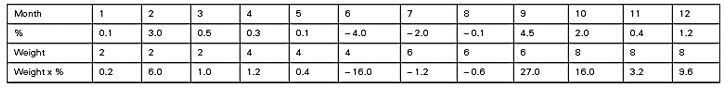
Suppose an investment has yielded a return over the year as follows:

[Arithmetic Mean of Periodic Returns]

The total of the monthly returns above (i.e., 0.1 + 3.0 + + 0.4 + 1.2) is 6%. The number of observations is 12. So arithmetic mean is 6% ÷ 12 = 0.5%.

3.   Frequency Distribution

In the above arithmetic mean each month’s return was given equal importance. An alternative is to give different weights to different periods.

Suppose we decide to give weights as follows:

With these weights, you can see that the more recent quarters have got higher weightage. You will also note that since each quarter has 3 months, the total of the weights for a full year is:

(2 x 3) +(4 x 3) +(6 x 3) +(8 x 3), i.e., 60

Let us apply the weights on the numbers we used for calculating arithmetic mean:

[Frequency Distribution]

The total of the (weight x %) row is 46.80%.

Time-weighted return is given by the formula:

Total (weight x %) ÷ Total (weights)

i.e., 46.80 % / 60 = 0.78 %

Thus, by giving higher importance to the recent good performances, the time weighted return is higher at 0.78%, as compared to the simple arithmetic mean of 0.50%.

While working with large volumes of data, it becomes cumbersome to do calculations using every data point. A shortcut that could be used is frequency distribution, which considers the frequency with which data points fall in different ranges of values. In the example used earlier for calculating the mean, for instance:

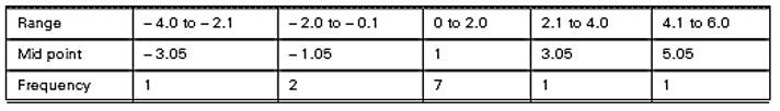
[Frequency Distribution-2]

The 12 observations are distributed as per the frequencies given above. When a frequency distribution is used, all the observations within the range are deemed to be equal to the mid-point of the range. This assumption simplifies all further data analysis. The validity of the assumption however depends on the data ranges, statistically referred to as “class intervals”, used.

Setting the data ranges is a very subjective and specialised exercise. If we set the ranges too narrowly (e.g., — 4.0 to — 3.8, — 3.8 to — 3.6, — 3.6 to — 3.4, and so on), then the number of ranges would end up being too many to give any benefit of using the frequency distribution. On the other hand, if the ranges are set too broadly (e.g., — 10.0 to — 0.1, 0 to 10.0 and so on), then the mid-point may not be truly representative of the underlying data.

4.   Mode

Suppose we have a sequence of returns like the following:

1%, 2%, — 1%. 3%. 2%, —3%, 2%, 5%, —3%, 2%, 2%

The most common occurrence among these 11 values is 2%, which occurs 5 times in the above sequence. The most frequently occurring data point is called the mode.

While deciding on the Unique Selling Proposition to offer on a mutual fund scheme, the issuing company would look at the most frequently liked feature, i.e. the mode, where the data points would be the single most liked feature in a scheme, ascertained from a sample of investors. If more investors prefer a 51:49 mix of debt and equity in a balanced scheme, then the scheme would be offered with 51:49 as the target asset allocation.

5.   Median

Median is the mid-point of the series, determined after the observations are ordered sequentially. The same sequence of returns used for the mode could be re-ordered as follows:

—3%, —3%, —1%, 1%, 2%, 2%, 2%, 2%, 2%, 3%, 5%

The midpoint of the series of 11 observations would be the 6th observation, i.e. 2%.

Suppose we want to determine out-performers of mutual fund schemes, we could use an average performer as a standard. There would then be some schemes which would have performed better, while others would have performed worse. If the arithmetic mean were to be used as the average, it could get highly influenced by a few schemes that show extremely good, or poor, performance. Instead, if the median is used, then an equal number of schemes would be better or worse than the average.

On account of the cumbersome process of having to re-order the observations so that they fall into a sequence, median is less commonly used.

6.   Expected Value / Volume Weighted Mean

In a world of uncertainty, it is difficult to make predictions; yet there is no shortage of “views”. At times, the number of views is more than the number of people from whom you seek the view!

Let us consider an example.

Television channels often seek the views of research analysts on the profits they expect companies to declare. Suppose the table on next page gives the views of different analysts on the expected profits of a company:

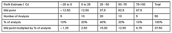
[Expected Value - Volume Weighted Mean]

Expected value of profits based on the volume weighted mean of analyst estimates is 37.50 crore. Similarly, expected value of returns from the market or a scheme can be determined.

7.   The Role of Dividend

Whenever a dividend is declared, the NAV of a mutual fund goes down because the dividend amount no longer belongs to the scheme, it belongs to the investors. The reduced NAV, immediately after a dividend distribution is referred to as “Ex-Dividend NAV”. If we calculate returns based only on the movement in NAV, it can lead to an understatement of return, whenever a dividend is paid or re-invested.

However, if a scheme has a growth option, i.e. where no dividends are declared, then the earnings would be fully reflected in the NAV. In such cases, the simple return can be calculated based on change in NAV, subject to the issues related to compounding.

8.   Total Return of a Mutual Fund

Total return is calculated like simple return, but the dividend distribution is added to the closing NAV. Suppose the NAV of a scheme has grown from Rs.10 to Rs.12 during a period of a year, where dividend of Rs.1 per unit was paid.

Simple return, we saw earlier, is:

Rs. (12-10) / Rs.10 = 0.2, i.e. 20 %.

Total return is:

Rs.(12 + 1 – 10) / Rs.10 = 0.3, i.e. 30 %

Thus, unlike simple return, total return includes the dividends paid. So it is a superior measure of return. However, the other weakness of simple return, namely no compounding, is a problem with total return too.

Further, we know that receiving a dividend towards the beginning of any period is more valuable (since it can earn interest if that dividend is deposited in a bank) than the same dividend received towards the end of the period. This time value of the dividend needs to be considered while calculating returns. In the above example, total return would be 30 %, irrespective of whether the dividend of Rs.1 was received at the beginning of the period or the end of the period. This is a serious weakness of the total return calculations.

9. Compounded Annual Growth Rate (CAGR) in Mutual Fund

If the NAV of the growth option of a scheme (which does not declare a dividend) grows from Rs.10 to Rs.12 over a 2-year time period, the CAGR can be calculated using the compound interest formula :

CAGR Formula:

[(CAGR) in Mutual Fund]

Thus, in the above example, CAGR would amount to:

(12/10) ^(½) = 9.54%

In the earlier IDBI Deep Discount Bond example, where 2,7OO was to grow into 1 lakh over 25 years, the CAGR amounts to 15.54% — a far cry from the simple return of 144% when inappropriately based on simple interest.

10.  CAGR with Re-investment of Dividend

In a situation where dividend is distributed, the CAGR is worked out on the following basis:

>        Assume that any dividend declared by a scheme is re-invested in the same scheme at the ex-dividend NAV.

>        On the above basis, calculate growth in number of units during the period for which returns are being calculated.

> Opening number of units multiplied by opening NAV would give opening wealth.

> Closing number of units multiplied by closing NAV would give closing wealth.

>        Use compound interest formula to determine the CAGR between the opening and closing wealth.

The calculations are shown in the example that follows. CAGR is a superior measure because it considers the dividend distribution (unlike simple return), and is also sensitive to the timing of such distribution (unlike total return). It also assumes that the dividend is re-invested in the same scheme. This is a more appropriate assumption for understanding the scheme’s return than an assumption that money is deployed somewhere else.

As discussed earlier, it is mandatory to use compounded return (CAGR) to disclose information in advertisements and offer documents if the period under consideration is more than a year.

Example

On 1 January 1998, the NAV of an equity scheme of the BCCI Mutual Fund was Rs. 10. It rose to Rs.30 by 1 January 2000. The scheme paid a dividend of Rs.1 per unit on 1 January 1999, and a further dividend of Rs.1 per unit on 1st January 2000. The ex-dividend NAV was Rs.20 on 1 January 1999. What is the return during the period 1998-99, 1999-2000 and 1998-2000?

For easy calculations, let us assume that the investor started with 18,000 units ii the scheme. (Whatever the initial number of units we assume, the calculated returns would be the same.)

The movement lithe vie of the scheme s as follows:

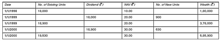
[CAGR with Re-investment of Dividend]

The period 1998-99 being exactly 1 year, we can calculate simple returns as follows:

Rs. (3,78,000 – 1,80,000) / Rs.1,80,000 = 1.1 i.e. 110%

Similarly, the period 1999-2000 being exactly 1 year, we can calculate simple returns as follows:

Rs. (5,85,900 – 3,78,000) / Rs. 3,78,000 = 0.55 i.e. 55%

The period 1998-2000 is more than 1 year.

Simple return (cumulative aggregate) during the period:

Rs. ( 5,85,900 – 1,80,000) / Rs. 1,80,000 = 2.255 i.e. 225.5%

Simple return (average annualised) for the 2 yeas is:

225.5% /2 = 112.75 %

The CAGR can be worked out using the formula:

Rs. (5,85,900 / 1,80,000) ^(1/2) - 1

Interestingly,  the same formula applied for 1998-99 would be:

Rs. ( 3,78,000 / 1,80,000) ^(1/1) – 1 = 1.1 = 110%

Similarly, the same formula applied for 1999-2000 would be :

Rs. (5,85,900 / 3,78,000) ^(1/1) – 1 = 0.55 = 55%

This confirms that when the period is exactly a year, the simple return is exactly equal to CAGR.

11.  XIRR (Extended Internal Rate of Return) of Mutual Fund

CAGR calculations for investors can be cumbersome, particularly when they have done multiple transactions of sale and re-purchase during a period. If the investor wants to know what return she earned from a scheme during such a period of multiple transactions, CAGR can become a nightmare. Further, for every dividend distribution, the analyst would also require the ex-dividend NAV. XIRR comes in handy here.

XIRR, a financial function available in MS Excel software. The formula is “XIRR(cell range of cash flows, cell range of timing of these cash flows). Thus, the formula captures information on the timing of various cash flows during the holding period of the investment. (Please note that the formula varies from the “IRRM function in MS Excel, where information on the cash flow is captured, but not the timing of these flows).

As seen earlier, CAGR is calculated assuming re-investment at ex-dividend NAV. On the other hand, the XIRR function in MS Excel presumes re-investment at the internal rate of return itself. The cash flows used for the XIRR calculations should therefore not consider increase in the number of units on account of reinvestment of dividend. The cash flows for the earlier example were:

The XIRR would give an annualised return of 81.14 %, which is marginally different from the CAGR of 80.42 %. This difference is on account of the different principles underlying CAGR and XIRR, namely reinvestment at ex-dividend NAV (in the case of CAGR) versus re-investment at the internal rate of return (in the case of XIRR). How does this difference in principles affect us?

>>        It is not always possible to re-invest moneys at the internal rate of return. Therefore, investors need to be cautious whenever the value of XIRR turns out to be too high. They need to ask themselves, “Will I be able to re-invest the moneys I receive on the investment, at the XIRR rate?” If the answer is no, then it would be better to avoid using the XIRR.

>>        In some situations, MS Excel will not give a valid answer for XIRR. This happens when there are too many investment and disinvestment transactions, on account of which the pattern of cash flows keeps changing from positive to negative and back. In such situations, one has to use CAGR only.

The assumption, which XIRR makes, that the re-investment rate would remain constant throughout the period of review, is obviously mistaken. On the other hand, CAGR provides for differential performance during the period of review. For instance, our earlier calculations were based on the first dividend being re- invested at 20, and the second dividend being re-invested at 30.

On account of these reasons, the CAGR is a fundamentally stronger method of measuring return. SEBI insists that statutory information from the AMC be disclosed on the basis of CAGR. However, specific calculations for investors are made by both fund houses and distributors on the basis of XIRR.

12.  Rolling Returns of Mutual Fund

Investors often like to know the returns for various periods of 7 days or 1 month or some such period. These are called “rolling returns”.

For example, the return from 1 October 2005 to 8 October 2005 represents a 7- day return. Similar calculation of returns from 2 October 2005 to 9 October 2005, 3 October 2005 to 10 October 2005, and so on, are called “7-Day Rolling Returns”.

Equity returns are highly volatile, when we view them as daily returns. But, when we look at equity returns over longer time periods, the rolling return charts look much more stable.

Debt investments earn interest each day. The longer the period that a person holds on to a debt investment or debt fund, greater would be the interest income available for setting off losses arising out of change in value of securities. On account of this influence of interest income (called “accrued income”), if the rolling returns for a debt scheme are plotted in a graph, the 1 -day rolling returns would vary far more significantly (i.e., be more volatile) than 7-day rolling returns, which, again, would vary more significantly than rolling returns for periods longer than 7 days.

It is often easier to convince an investor to invest in a mutual fund scheme by demonstrating the low volatility of 30—day rolling returns (for debt schemes) or 3- year rolling returns (for equity schemes). Of course, this pre-supposes that the investor is prepared to hold the investment for at least 30 days or 3 years, as the case may be.

13. Mutual Fund Load Adjusted Returns

The calculations given above were at the scheme level. NAV was used as a determinant of the scheme’s performance.

If an investor has paid an entry load (invested at more than NAV — no longer permitted) or incurred an exit load I contingent deferred sales load (recovered less than NAV on exit), then the investor’s actual returns would be less than the scheme’s performance calculated based on NAV.

Thus, in the above example if an exit load of Rs.1.50 was applicable on 1 January 2000, then the investor would recover only Rs.28.50 per unit — not Rs.30.00 per unit. In that case, her closing wealth is only Rs.5,56,605, giving a CAGR of 75.85 % for the two-year period.